
Statistics basic concepts
This is my personal cheatsheet and tutorial for statistics. It is far from being a complete introduction, the main goal is to have a centralized resource where one can quickly remember or access more detailed resources. Many paragraphs are excerpts from the linked Wikipedia articles in the associated section. \(\def\mean#1{\bar #1} \DeclareMathOperator{\EV}{\mathbb{E}} \DeclareMathOperator{\Prob}{\mathbb{P}}\)
Concepts of Research Methods
Construcs
Something hard to measure, that you’ll have to define how to measure.
Operational Definition
It’s how you will measure a given construct.
Sample
A sample is a (sub)set of elements from a population of interest.
When it is not feasible to directly measure the value of a population parameter (e.g., unmanageable population size), we can infer its likely value using a sample (a subset of manageable size).
Note: make sure to distinguish between the terms sample size and number of samples. Use the former to describe the number of elements in a sample, and the latter to refer to the number of different samples (each constituted of many elements), if that is the case.
Parameter vs Statistic
A parameter refers to a quantity the defines the actual, entire population (the original distribution) of interest. In contrast, a statistic refers to a quantity computed using values in a sample (part of the population).
A statistic can be used to estimate a population parameter, to describe a sample, or to evaluate a hypothesis. When used to estimate a population parameter, it is called an estimator.
Relationships vs Causation
Relationships can be shown by observational studies (eg. by seeing a point distribution). Causation, however, has to be found through controlled experiments.
Measures of central tendency
Mode
The value at which frequency is highest.
The mode doesn’t really represent the data well because:
- It’s not affected by all scores in the dataset;
- It changes radically depending on the sample;
- We can’t really describe the mode by an equation.
Median
The value in the middle of the distribution.
(If there are an even number of elements, the median will be the average of the two in the middle.)
The median is more robust to outliers than the mean. It is therefore the best measure of central tendency when dealing with highly skewed distributions.
Mean (expected value)
The weighted average, or expected value.
- Population mean: $\mu$
- Sample mean: $\mean{x}$ (can be used to estimate $\mu$)
- The mean is sensitive to outliers
- The law of large numbers states that as a sample size grows, its mean gets closer to the average of the whole population.
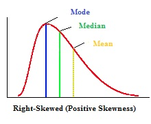
The mean is always pulled towards the longest tail of the distribution, in relation to the median.
Variability of data
Range
Range = MaxValue - MinValue
Interquartile Range (IQR)
IQR is the distance between the 25% and the 75% higher measure of the data.
IQR = Q3 - Q1
Problem with Range and IQR: neither takes all data into account.
Outlier
An observation point that is distant from other observations.
Values below (Q1 - 1.5*IQR) or above (Q3 + 1.5*IQR) are usually considered outliers.
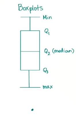 Outliers are represented as dots in a boxplot.
Estimators, Bias and Variance
(from a machine learning point of view)
Point Estimation
Point estimation is the attempt to provide the single “best” prediction of some quantity of interest. A point estimator or statistic is any function of the data:
\[\boldsymbol{\hat \theta}_m = g(\boldsymbol{x}^{(1)},...,\boldsymbol{x}^{(m)}).\]The definition does not require that $g$ return a value that is close to the true $\boldsymbol{\theta}$ or even that the range of $g$ is the same as the set of allowable values of $\boldsymbol{\theta}$.
Bias
Bias measures the expected deviation from the true value of the function or parameter. The bias of an estimator is defined as:
\[\text{bias}(\boldsymbol{\hat\theta}_m) = \EV(\boldsymbol{\hat\theta}_m) - \boldsymbol{\theta}\]where the expectation is over the data (seen as samples from a random variable).
Variance and Standard Deviation
Variance provides a measure of the deviation from the expected estimator value that any particular sampling of the data is likely to cause.
We call deviation a measure of difference between the observed value of a variable and some other value, often that variable’s mean. We calculate the variance by taking the mean of squared deviations:
\[\sigma^2 = \sum_{i=1}^{n} \frac{(x_i - \mean{x})^2}{n}\]The standard deviation is simply the root square of the variance. One interesting characteristic of the standard deviation is the 68–95–99.7 rule.
Bessel’s Correction (unbiased estimator of the population variance)
You use $(n - 1)$ instead of $(n)$ to calculate the standard deviation when estimating the standard deviation for the population from a sample.
\[\sigma \approx s = \sqrt{\sum_{i=1}^{n} \frac{(x_i - \mean{x})^2}{n - 1}}\]Using the sample standard deviation (s) corrects the bias in the estimation of the population variance. It also partially corrects the bias in the estimation of the population standard deviation. However, the correction often increases the mean squared error in these estimations.
These [1, 2] short videos try to bring some intuition on why to use $(n - 1)$ instead of $(n)$.
The problem is that, by using the estimate $(\mean{x})$ instead of the actual population mean $(\mu)$, we create bias in the estimated variance by underestimating it, because $(\mean{x})$ is the value that minimizes $\sum_{i=1}(x_i - \mean{x})^2$, whereas $\mu$ could be any other value that makes it larger.
Using $n-1$ in $s^2$ to estimate $\sigma^2$ fixes this bias, making $s^2$, on average, equals $\sigma^2$ (unbiased estimator).
Z-Score
The Z-Score (aka standard score) maps a sample $x_i$ to how many standard deviations $\sigma$ it is from the mean $\mu$:
\[z_i = \frac{x_i - \mu}{\sigma} \ \ \ \implies \ \ \ x_i = \mu + z_i \cdot \sigma\]By its definition, the z-score is a dimensionless quantity. It can mapped directly to a percentile when you know the shape of the distribution (or, in case you do not, to weaker bounds using Chebyshev’s inequality).
The Bias vs Variance Tradeoff
How to choose between two estimators: one with more bias and another with more variance? The most common way to negotiate this trade-off is to use cross-validation. Alternatively, we can also compare the mean squared error (MSE) of the estimates:
\[\begin{align} \text{MSE} & = \EV \left[ \left( \hat\theta_m - \theta \right)^2 \right] \\ & = \text{Bias} \left( \hat\theta_m \right)^2 + \text{Var} \left( \hat\theta_m \right)^2 \end{align}\]The relationship between bias and variance is tightly linked to the machine learning concepts of capacity, underfitting and overfitting.
Sampling distributions
The sampling distribution is the probability distribution of the values a statistic (e.g., sample mean or sample variance) can take on.
Standard Error
The standard error of a statistic corresponds to the standard deviation of its sampling distribution. If the parameter or the statistic is the mean, it is called the standard error of the mean (SEM).
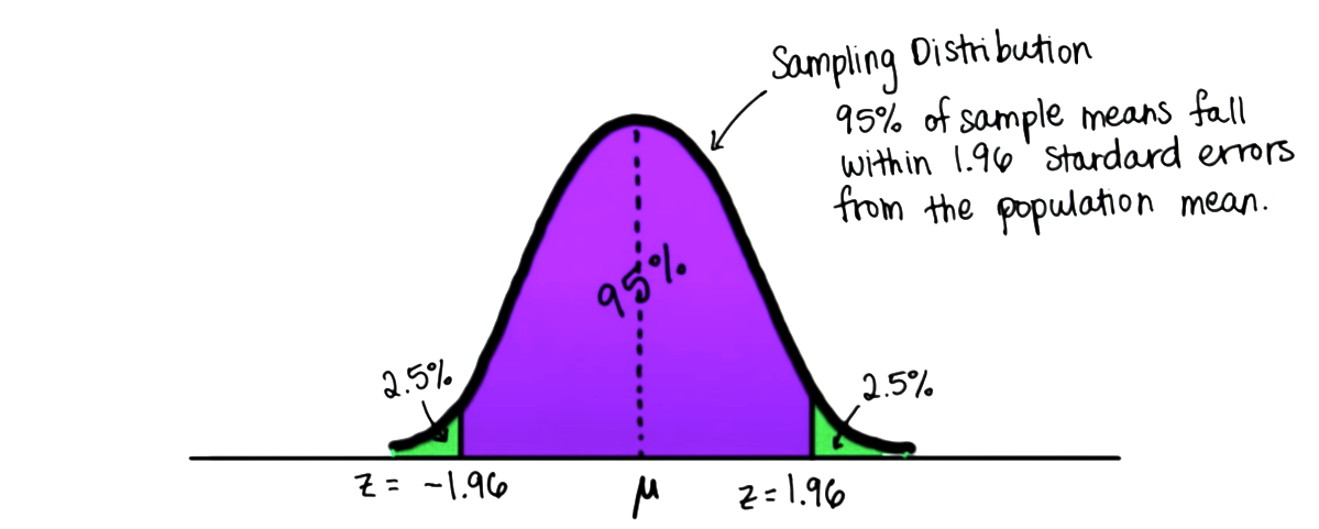 Depiction of distribution sampling, taken from [2].
Standard Error of the Mean (SEM) $\sigma_{\bar{x}}$
The SEM quantifies the precision of the mean, i.e., it measures how far the sample mean is likely to be from the true population mean. In other words, the SEM is the standard deviation of the distribution that defines the values of the sample mean we will observe, for each sample of size $n$ we take from the population.
Since $\sigma$ is seldom known (to calculate it we’d have to make lots of experiments, finding many different values for the mean, and calculating its standard deviation), the SEM is usually estimated by using the sample standard deviation:
\[\text{SEM} = \sigma_{\bar{x}} = \frac{\sigma}{\sqrt{n}} \approx \frac{s}{\sqrt{n}}\]The proof of the relationship between the SEM, the standard deviation of the population $\sigma$, and the sample size $n$ is shown below (reference). The first step is allowed because the $X_i$ are independently sampled, so the variance of the sum is just the sum of the variances.
\[\text{Var}\bigg(\frac{\sum_{i=1}^{n}{X_i}}{n}\bigg) = \frac{1}{n^2}\text{Var}\bigg(\sum_{i=1}^{n}{X_i}\bigg) = \frac{1}{n^2}\sum_{i=1}^{n}\text{Var}\bigg({X_i}\bigg) = \frac{1}{n^2}\sum_{i=1}^{n}{\sigma^2} = \frac{\sigma^2}{n}\]We can use the SEM to interpret different populations and see if there is evidence that there are differences or similarities between them:
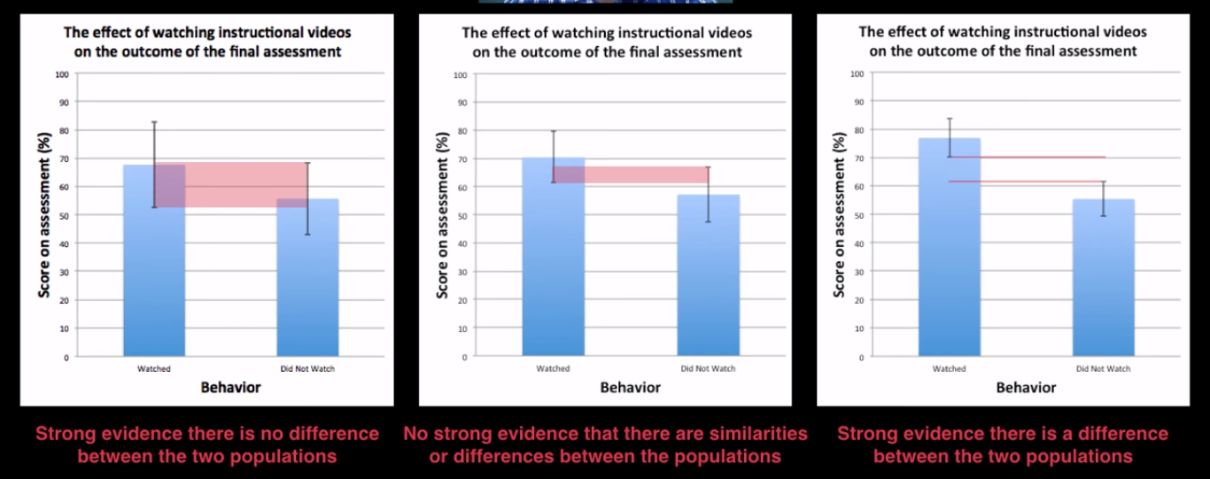 How the standard error of the mean helps us interpret populations, from this YouTube video.
We can also use the relationship between the SEM and the sample size $n$ to define how many elements we need in our sample to achieve a desired level of statistical significance.
Link: simulation applet to explore aspects of sampling distributions.
Margin of error and confidence interval
Given a confidence level $\gamma$ chosen by the investigator, a confidence interval has a probability $\gamma$ of containing the true underlying parameter. In turn, the margin of error (MOE) corresponds to how distant from the interval mean its margins are (i.e., half the width of the confidence interval).
A line of inferential reasoning one could use to define a confidence interval is:
- We know the properties of the sampling distribution, e.g., we know that the probability ofh yoaving the sample mean $\bar{x}$ fall between 1.96 standard errors $\sigma_{\bar{x}}$ from the population mean $\mu$ is 95%.
- Thus, we know that $\mu$ is at most $1.96\sigma_{\bar{x}}$ away from $\bar{x}$ with 95% confidence.
- We calculate $\sigma_{\bar{x}}$ and arrive at our confidence interval.
- If we know $\sigma$, then it is straightforward;
- If we don’t know $\sigma$, we estimate it using the sample standard deviation $s$.
Which gives us the general formula:
\[\text{CI} = \left( \bar{x} - z_{\gamma}\frac{\sigma}{\sqrt{n}} \ , \ \bar{x} + z_{\gamma}\frac{\sigma}{\sqrt{n}} \right)\]Statistical hypothesis testing
Null and alternative hypothesis
The null hypothesis $H_0$ is a default position that there is no relationship between two measured phenomena or no association among groups. It is usually contrasted with an alternative hypothesis $H_1$, a new theory.
Statistical hypotheses are usually formulated in terms of a test statistic, a one-value numerical summary of a dataset, defined in a way that distinctions between the two hypotheses can be made. The test statistic must be such that its sampling distribution and, consequently, p-values can be calculated.
It is common to define $H_0$ as the test statistic being the same (precisely, not significantly different) for the different groups/conditions we are examining, and the alternative hypothesis as the group/conditions having significantly different values of the test statistic:
\[\begin{align} H_0 : \mu_1 = \mu_2 \quad , \quad H_1 & : \mu_1 \neq \mu_2 \quad \text{(two-tailed test)} \\[0.8ex] H_0 : \mu_1 \le \mu_2 \quad , \quad H_1 & : \mu_1 \gt \mu_2 \quad \text{(one-tailed test)} \\ H_0 : \mu_1 \ge \mu_2 \quad , \quad H_1 & : \mu_1 \lt \mu_2 \quad \text{(one-tailed test)} \\ \end{align}\]Notice that the boundaries between $H_0$ and $H_1$ are defined in terms of statistical significance, not in the strict mathematical sense. For instance, if we found out that the (true) test parameter of the experimental group would be slightly but not significantly different than that of the control group, we would still consider $H_0$ as the correct hypothesis.
Two-tailed (non-directional) tests are more general (more conservative); one-tailed (directional) tests are used when we expect a direction of the treatment effect (e.g., we want to compare a new webpage interface with an established one and we care only about assessing if the change will improve what is currently deployed).
p-value
p-value refers to the probability of obtaining test results equals to or more extreme than the actual observations, under the assumptions that the null hypothesis $H_0$ is correct.
- $\text{p-value} = \Prob(T \ge t \mid H_0)$ for one-sided, right tail test.
- $\text{p-value} = \Prob(T \le t \mid H_0)$ for one-sided, left tail test.
The smaller the p-value, the less likely $H_0$ holds, and the higher the statistical significance is said to be.
Statistical significance
In simple words, statistical significance is a determination by an analyst that the results in the data are not explainable by chance alone [3].
More precisely, given a significance level $\alpha$ (chosen before the study) and the p-value $p$ of a result, the result is statistically significant when $p < \alpha$.
Values for $\alpha$ are usually set to 5% or lower, depending on the field of the study and what probability is considered “unlikely” to occur.
Other concepts
i.i.d.
Independent and identically distributed random variables refers to a collection of random variables that are mutually independent from each other and sampled from the same probability distribution.
Central limit theorem
The central limit theorem states that, when i.i.d. random variables are summed, the resulting distribution tends toward a normal distribution, as the sample size grow, even if the original variables themselves are not normally distributed.
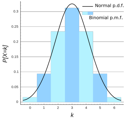
Continuity correction
Continuity correction are used when approximating a discrete random variable with a continuous one [ref].
Type I and Type II errors
Type I error is rejecting a true null hypothesis; Type II error is not rejecting a false null hypothesis. (Type I and type II errors - Wikipedia)
References
- Wikipedia
- Udacity course on Statistics
- https://www.investopedia.com/terms/s/statistically_significant.asp